19  Ensemble Methods

19.1 Introduction

In predictive modelling, a single model often struggles to capture the full complexity of real-world data. Even well-constructed machine learning models have inherent weaknesses:

• Some may be overly simplistic, failing to capture important relationships;

• Others may be overly sensitive to training data, leading to poor generalisation.

Note

Ensemble learning, the focus of this chapter, offers a powerful solution to this issue by combining multiple models to achieve better predictive performance than any individual model alone.

The effectiveness of ensemble methods is based on three key principles:

• the bias-variance trade-off;
• model diversity; and
• aggregation strategies.

Each of these plays a role in ensuring that ensemble models not only make accurate predictions but also generalise well to unseen data.

19.1.1 Bias-variance tradeoff

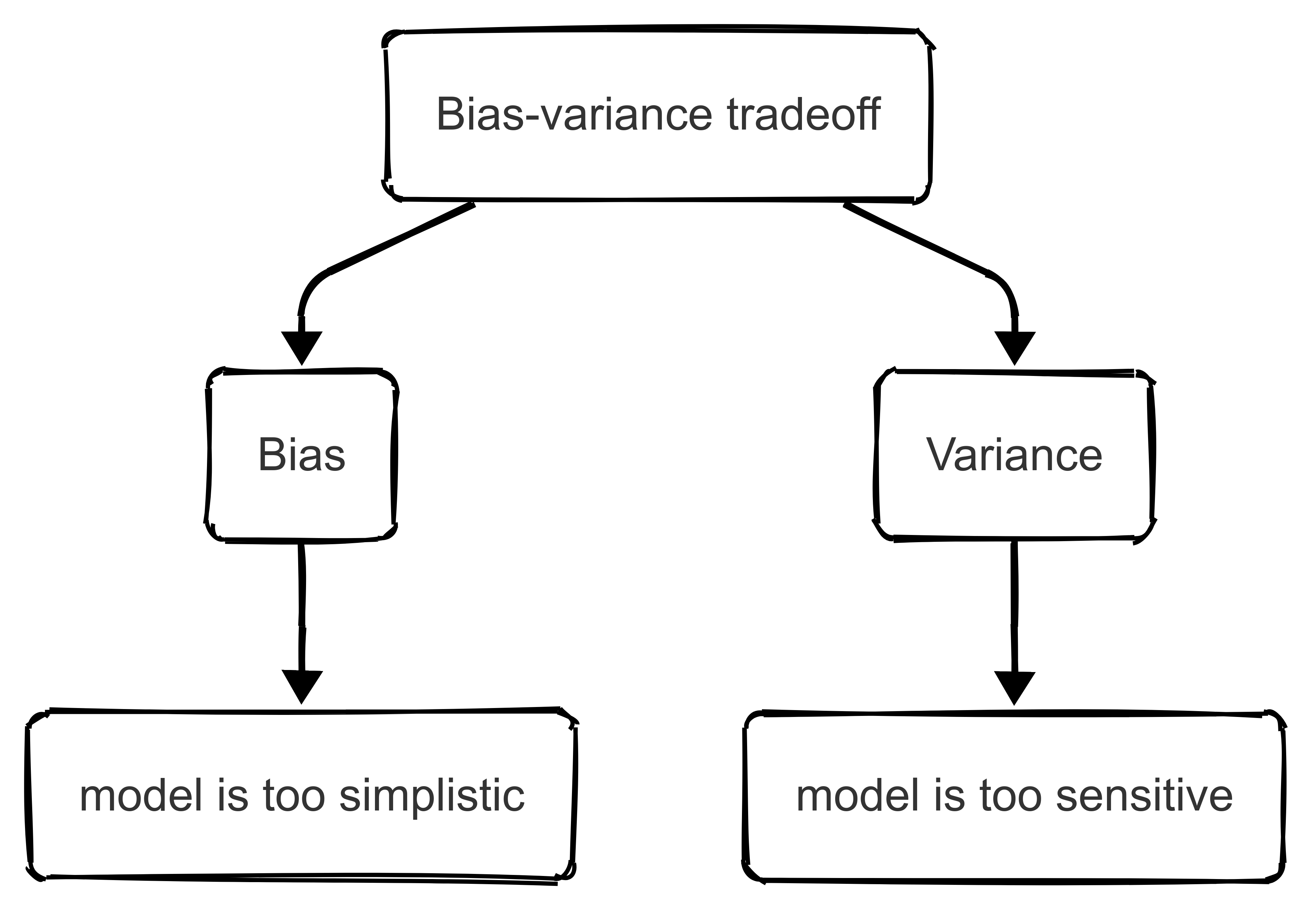
One of the fundamental challenges in machine learning is the bias-variance trade-off. This describes the balance between a model’s ability to make accurate predictions and its ability to generalise to new data.

Bias refers to systematic errors that arise when a model is too simplistic and unable to capture underlying patterns in the data.

• High-bias models (such as basic linear regression models) make strong assumptions about the relationships between variables and often fail to capture complex interactions.
• As a result, they tend to underfit the data, meaning that their predictions are consistently inaccurate across different datasets.

On the other hand, variance refers to the sensitivity of a model to fluctuations in the training data.

• A model with high variance may perform really well on the training data but struggle when presented with new, unseen data.
• This is because it has learned the ‘idiosyncrasies’ of the training set rather than the broader patterns that generalise to other situations.

High-variance models (such as deep neural networks or high-degree polynomial regression), on the other hand, are prone to overfitting, meaning they memorise the training data rather than extract meaningful patterns.

Important

Ensemble learning gives us a structured way to mitigate the bias-variance trade-off. By combining multiple models, ensembles reduce variance without necessarily increasing bias.

The underlying principle is that individual models make different types of errors, and when their predictions are aggregated, the overall error rate decreases.

This is particularly useful in contexts where data can be highly variable, and influenced by numerous contextual factors.

For example, in injury prediction models, a single decision tree may either oversimplify the relationship between workload and injury risk (leading to high bias) or overfit to specific player data (resulting in high variance).

By using an ensemble of decision trees, such as a random forest, our prediction model can capture complex relationships while avoiding the pitfalls of overfitting.

19.1.2 Model diversity

For an ensemble model to be effective, the individual models within it must be diverse.

If all models make similar predictions and errors, then combining them provides little benefit!

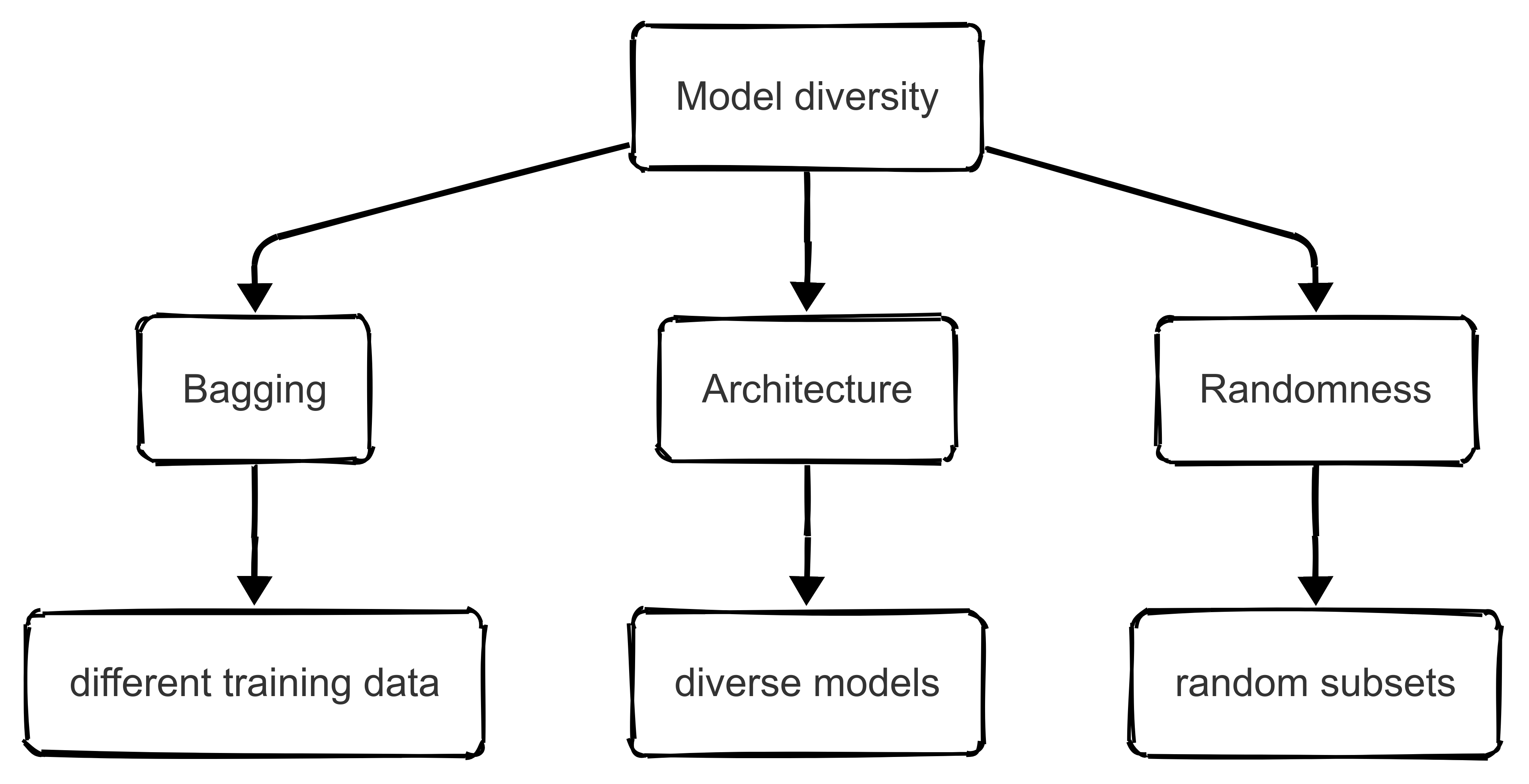
Model diversity ensures that the errors of one model are counterbalanced by the strengths of another, leading to more accurate and stable predictions. There are several ways we can introduce diversity into an ensemble, each of which plays a crucial role in improving performance.

Bagging

One approach to achieving diversity is to train models on different subsets of the data. This is the fundamental principle behind bootstrap aggregating, commonly known as “bagging”.

In bagging, multiple models are trained independently on randomly drawn subsets of the training data. Since each model is exposed to slightly different information, it develops a unique decision boundary. When the predictions of these diverse models are averaged, the overall variance of the ensemble is reduced, leading to more stable performance.

Model architecture

Another way to ensure diversity is by incorporating different model architectures. Instead of using multiple instances of the same model type, ensembles can be constructed using a combination of different models.

• For example, in game outcome prediction, a logistic regression model might be trained on historical win-loss records, a neural network might analyse player statistics, and a gradient boosting model might incorporate external factors such as weather conditions and team travel distances.

• Each of these models captures different aspects of the problem, and when their outputs are combined, the final prediction benefits from a broader range of insights.

Randomness

Diversity can also be introduced by injecting randomness into the model-building process. Some ensemble methods, such as random forests, achieve this by selecting different subsets of features for each tree within the ensemble.

This approach ensures that individual models are not overly reliant on specific features, making the ensemble more robust to variations in the data.

19.1.3 Aggregation strategies

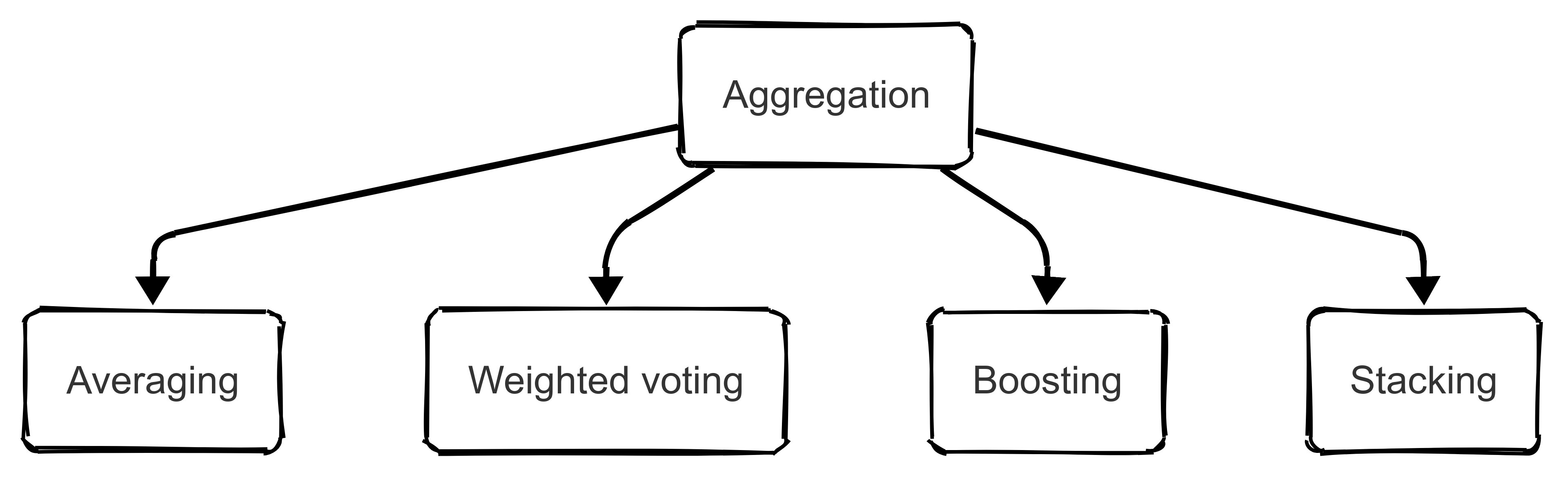
Once multiple diverse models have been trained, their predictions must be aggregated to produce a final output. The way in which these predictions are combined plays an important role in determining the effectiveness of the ensemble.

Different aggregation strategies exist, each suited to different types of predictive tasks.

Averaging

One of the simplest aggregation strategies is averaging, which is the foundation of bagging-based approaches such as random forests.

When an ensemble produces multiple predictions, taking the average of those predictions reduces variance and leads to a more stable and reliable outcome.

This is particularly useful in regression problems (e.g., predicting player workload metrics in football) where combining multiple estimations results in a more accurate assessment of how far a player is likely to sprint during a match.

Weighted voting

A more sophisticated approach to aggregation involves weighted voting, where models are assigned different levels of importance based on their performance.

In this method, models that have historically made more accurate predictions are given greater influence in the final decision.

This strategy is often applied in classification problems (such as predicting the outcome of a match).

For example, if a logistic regression model based on historical win rates has proven to be highly accurate, it may be assigned a greater weight than a random forest model that considers in-game shot effectiveness.

By optimising how much each model contributes to the final prediction, weighted voting improves the overall accuracy of the ensemble.

Boosting

Another widely used strategy is boosting, which involves training models sequentially so that each new model focuses on correcting the errors of the previous ones.

Unlike bagging, which trains models independently, boosting adapts based on previous mistakes, progressively improving the predictive performance. Gradient boosting models, such as XGBoost, are particularly effective in reducing bias while maintaining low variance.

In sport analytics, boosting could be useful in tasks that require nuanced pattern recognition (e.g., predicting the success probability of a basketball shot).

Since boosting focuses on refining difficult-to-predict cases, it is well suited for problems where certain events, such as three-point shots under defensive pressure, are particularly challenging to model.

Stacking

A more complex but highly effective aggregation strategy is stacking, also known as “meta-ensemble” learning.

In stacking, multiple models make independent predictions, and a higher-level meta-model is trained to learn how to best combine those predictions. The meta-model determines which models are most reliable under different circumstances, producing a final output that leverages the strengths of all base models.

In player valuation analysis, for instance, stacking could be used to combine insights from models trained on historical transfer fees, player performance statistics, and market trends.

Each model contributes different information, and the meta-model learns how to weight their contributions to generate a more precise valuation.

19.2 Advanced Bagging and Random Forests

As noted above, bagging (bootstrap aggregating) is a powerful ensemble learning technique that improves predictive accuracy by reducing variance and enhancing model stability.

Remember: the fundamental idea behind bagging is to generate multiple versions of a base model, each trained on a slightly different subset of the training data.

These individual models then contribute to a final aggregated prediction, which is typically obtained by averaging for regression tasks or by majority voting for classification tasks.

One of the most widely used applications of bagging is the random forest algorithm, which extends traditional decision trees by introducing additional randomness and robustness.

This section explores the inner workings of bagging, with a specific focus on random forests, while also discussing hyperparameter tuning, feature importance evaluation, and practical applications in sports analytics.

19.2.1 The inner workings of bagging algorithms

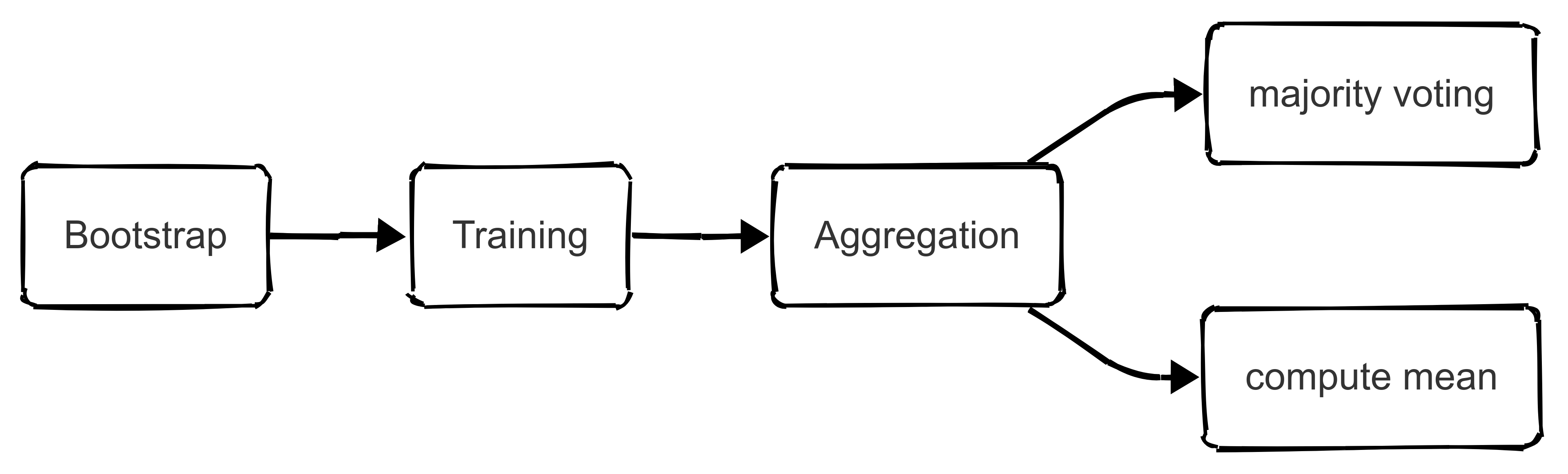
Bagging works by constructing multiple base learners from re-sampled training data.

• The process begins by creating bootstrap samples, where each sample is drawn randomly from the original dataset with replacement. This means that some observations appear multiple times in a given bootstrap sample, while others are omitted.
• Each base model is then trained independently on its respective sample, resulting in a diverse set of models that capture different aspects of the data.
• Since each model sees a slightly different dataset, they develop unique decision boundaries, which helps mitigate overfitting to specific training instances.
• Once all models have been trained, their outputs are aggregated.
  • In regression tasks, this usually involves computing the mean of individual predictions, effectively smoothing out extreme errors and leading to a more stable and generalisable model.
  • In classification tasks, aggregation is typically performed using majority voting, where the most commonly predicted class among all models is selected as the final output. This approach significantly reduces variance while maintaining predictive accuracy.

Bagging is particularly well suited for high-variance models such as decision trees, which tend to be highly sensitive to fluctuations in the training data. By averaging multiple trees, bagging reduces the risk of overfitting while maintaining the flexibility and interpretability of decision tree-based models.

19.2.2 Random Forests: Enhancing bagging with feature randomisation

Random forests are an extension of bagging that introduce additional randomness during model training. In a standard bagging approach, each decision tree has access to the full set of input features when determining splits.

However, in a random forest, each tree is restricted to a random subset of features at each decision node. This additional layer of randomness forces individual trees to develop diverse decision rules, further reducing the risk of overfitting and improving the ensemble’s generalisation ability.

The key advantage of random forests is their ability to de-correlate individual trees, ensuring that the ensemble does not overly rely on a particular set of features. This makes random forests particularly useful for prediction tasks with numerous correlated features, such as predicting team performance stability in football or identifying injury risk factors in basketball.

Since different trees emphasise different combinations of predictors, the model captures a broader range of potential relationships, making it more robust to fluctuations in player statistics, environmental conditions, or opponent strategies.

19.2.3 Hyperparameter tuning for random forests

The performance of a random forest model depends heavily on the selection of key hyperparameters.

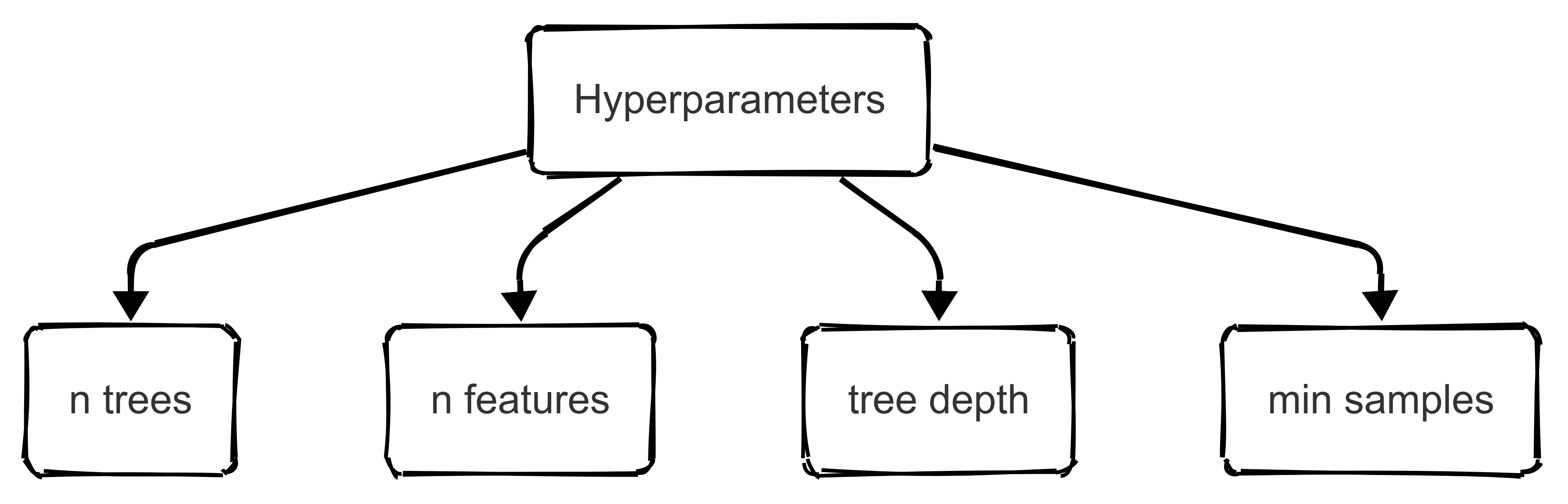
Proper tuning of these hyperparameters ensures that our model achieves an optimal balance between bias and variance, ultimately improving predictive accuracy. The most critical hyperparameters include:

Number of trees (n_estimators)

The number of trees in the ensemble affects both accuracy and computational efficiency. A larger number of trees generally improves performance by reducing variance, but after a certain point, the gains become negligible.

Note: typical values range from 100 to 500 trees, depending on dataset size and computational constraints.

Number of features per split (max_features)

This parameter determines how many randomly selected features each tree considers when determining a split. A lower value increases diversity among trees, reducing correlation between them and improving generalisation. In classification tasks, a common approach is to use sqrt(n_features), while in regression tasks, n_features / 3 is often a reasonable starting point.

Tree Depth (max_depth)

Limiting tree depth prevents excessive complexity and overfitting. Shallow trees generalise better but may underfit, while deep trees increase the risk of memorising training data. A good approach is to tune this parameter using cross-validation, especially in datasets where interpretability is important.

Minimum Samples per Split (min_samples_split) and Minimum Samples per Leaf (min_samples_leaf)

These parameters control how many observations are required to make a split or to form a leaf node. Higher values prevent the model from capturing noise in the data, making predictions more stable. In sport analytics, this could be applied to models predicting player workload, where outliers (e.g., extreme high-intensity performances) should not overly influence the model.

Bootstrap sampling (bootstrap)

By default, random forests use bootstrap sampling, meaning each tree is trained on a resampled version of the dataset. Disabling this (setting bootstrap=False) results in each tree seeing the full dataset, which can reduce variance further in some cases but at the risk of increasing overfitting.

Hyperparameter tuning is often performed using grid search or Bayesian optimisation, ensuring that the random forest model achieves the best possible performance for the given dataset.

19.2.4 Evaluating feature importance in random forests

One of the major strengths of random forests is their ability to quantify feature importance, providing insights into which variables are most influential in making predictions. Feature importance is typically computed based on mean decrease in impurity (MDI) or permutation importance.

Mean decrease in impurity

The mean decrease in impurity (MDI) approach evaluates how much each feature contributes to reducing uncertainty in the dataset. Features that frequently appear in important splits are assigned higher importance scores.

In sport analytics, this could be useful for identifying key performance indicators (KPIs) that determine player success. For instance, when predicting injury risk, a random forest model may reveal that minutes played per game, sprint distance, and high-impact collisions are the most predictive factors.

Permutation importance

Permutation importance, on the other hand, evaluates feature significance by randomly shuffling values for each feature and measuring the corresponding drop in model accuracy. This method provides a more robust assessment, especially when variables are correlated. In predicting team performance stability, for example, permutation importance might highlight that passing accuracy and defensive recoveries are stronger indicators than raw scoring statistics.

19.2.5 Application in sport analytics

Random forests could usefully be applied in sport analytics due to their flexibility, interpretability, and ability to handle complex relationships between variables.

For example, given a dataset containing player workload metrics, biometric data, and recent match performance, a random forest model can analyse which factors contribute most to injury likelihood. The model may reveal, for example, that players experiencing a high frequency of accelerations and decelerations are at increased risk of muscle injuries, allowing coaching staff to adjust training intensity accordingly.

19.3 Advanced Boosting Methods

19.3.1 Introduction

Boosting is a powerful ensemble learning technique that improves predictive accuracy by sequentially combining weak learners in a way that emphasises difficult-to-predict instances. Unlike bagging, which builds independent models in parallel and aggregates their predictions, boosting builds models sequentially, where each new model corrects the errors made by its predecessors.

Note

The key idea behind boosting is to iteratively refine predictions by focusing on misclassified instances, thereby reducing bias while maintaining low variance.

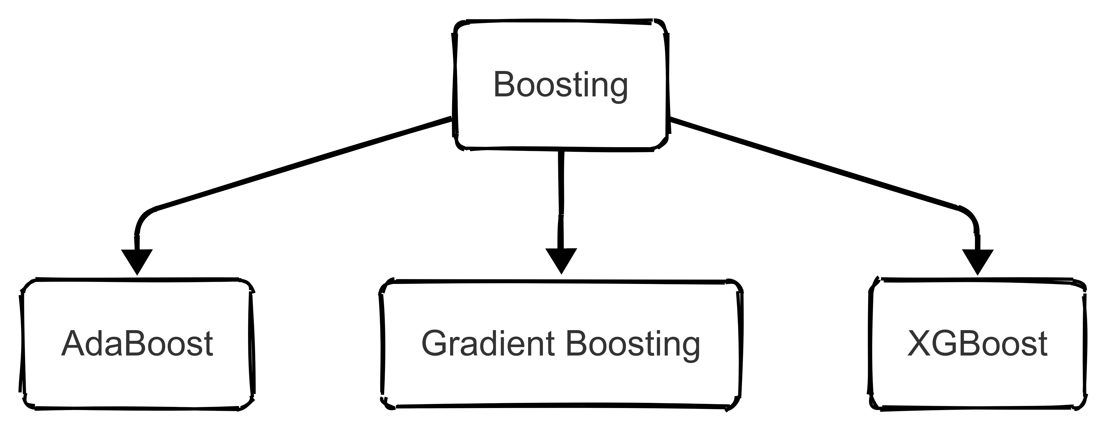
This section explores AdaBoost (Adaptive Boosting), Gradient Boosting, and XGBoost (Extreme Gradient Boosting). We’ll cover their mathematical foundations, optimisation techniques, hyperparameter tuning strategies, and applications in sport analytics.

19.3.2 AdaBoost: Adaptive Boosting and Its Mechanism

AdaBoost combines several weak classifiers into one strong classifier. It works as follows:

1. Initialise weights: Give equal initial weights (\(w_i\)) to each of the (N) training examples:

   \[ w_i = \frac{1}{N}, \quad i = 1, 2, \dots, N \]

2. Iterative Training: For each iteration (\(t = 1, 2, \dots, T\)):

   1. Train a weak classifier ( h_t(x) ) on the weighted dataset.

   2. Compute the classification error (\((\varepsilon\_t)\)):

   \[ \varepsilon_t = \sum_{i=1}^{N} w_i I(h_t(x_i) \ne y_i) \]

   where (\(I(\cdot)\)) is the indicator function, equal to 1 when (\(h_t(x_i) \ne y_i\)) and 0 otherwise.

3. Calculate Classifier Weight (\(( \alpha\_t )\)):

   \[ \alpha_t = \frac{1}{2} \ln\left(\frac{1 - \varepsilon_t}{\varepsilon_t}\right) \]

4. Update Example Weights: Increase weights for misclassified examples:

   \[ w_i \leftarrow w_i \exp\left(\alpha_t \, I(h_t(x_i) \ne y_i)\right) \]

   Then, normalize weights so they sum to 1:

   \[ w_i \leftarrow \frac{w_i}{\sum_{j=1}^{N} w_j} \]

5. Final Classifier: The final strong classifier combines all weak classifiers, weighted by their accuracy:

   \[ H(x) = \text{sign}\left(\sum_{t=1}^{T} \alpha_t h_t(x)\right) \]

Optimisation and hyperparameter tuning

AdaBoost primarily relies on the number of weak learners \(T\), which should be optimised to balance bias and variance. Too few iterations lead to underfitting, while too many can lead to overfitting, especially in noisy datasets. The learning rate, \(η\), can also be adjusted to control the influence of individual models.

19.3.3 Gradient Boosting: A generalised Boosting Approach

Gradient Boosting generalises the boosting approach, repeatedly training weak learners by fitting them to the residual errors of previous models.

Rather than weighting examples differently (as AdaBoost does), Gradient Boosting directly minimises a loss function by iterative improvement.

The algorithm works as follows:

• Initialisation: Begin by setting an initial prediction ( F_0(x) ) as a constant value minimizing the overall loss function:

\[ F_0(x) = \underset{c}{\arg\min} \sum_{i=1}^{N} L(y_i, c) \]

• Iterative Training: For each iteration (\(t = 1, 2, \dots, T\)):

• Compute Residuals: Calculate the residuals for each data point: \[ r_i^{(t)} = -\frac{\partial L(y_i, F_{t-1}(x_i))}{\partial F_{t-1}(x_i)} \]

• Fit a Weak Learner: Train a weak learner (\(h_t(x)\)) to predict these residuals (\(r_i\^{(t)}\)).

• Find Optimal Step Size (\((\gamma\_t)\)): Determine the best step size that minimises the loss function: \[ \gamma_t = \underset{\gamma}{\arg\min} \sum_{i=1}^{N} L(y_i, F_{t-1}(x_i) + \gamma h_t(x_i)) \]

• Update Model: Update the model by adding the new learner scaled by the step size: \[ F_t(x) = F_{t-1}(x) + \gamma_t h_t(x) \]

After (\(T\)) iterations, the final prediction function is given by (\(F_T(x)\)).

Hyperparameter Tuning and Optimisation

Gradient Boosting has several tunable hyperparameters:

• Learning rate (η): Controls the step size at each iteration. Lower values reduce overfitting but require more trees.

• Number of estimators (\(T\)): The number of boosting rounds. More trees improve performance but increase computational cost.

• Tree depth: Controls model complexity. Shallow trees prevent overfitting.

• Minimum samples per leaf: Prevents the model from memorizing noise by ensuring each leaf represents multiple samples.

19.3.4 XGBoost: Extreme Gradient Boosting and Its Advantages

Algorithmic enhancements in XGBoost

XGBoost is an optimised version of Gradient Boosting that introduces regularisation, parallel processing, and sparsity-aware split finding. The objective function combines loss minimisation and model complexity control:

\[ L=∑i=1NL(yi,y^i)+λ∣∣Θ∣∣+γT \]

where: \(L(y,y^)\) is the loss function (e.g., squared error for regression), λ∣∣Θ∣∣ is L2 regularisation to reduce overfitting, γT penalises the number of trees to prevent excessive model complexity.

XGBoost also introduces second-order optimisation, leveraging both the gradient and Hessian (second derivative) for better convergence.

Hyperparameter tuning in XGBoost

Max depth: Deeper trees capture more relationships but risk overfitting. Subsample ratio: Controls the percentage of training data used per tree, reducing correlation among models.

• Colsample_bytree: Limits the number of features used per tree to enhance generalisation.
• Gamma: Controls tree pruning; higher values encourage simpler models. -bLearning rate (η): Lower values improve generalisation but require more boosting rounds.

19.4 Stacking (Meta-modeling)

Stacking, also known as stacked generalisation, is a powerful ensemble learning technique that enhances predictive accuracy by combining multiple models through a higher-level meta-model.

Unlike bagging and boosting, which aggregate predictions using simple averaging or weighted voting, stacking explicitly learns how to combine the outputs of different models using a meta-learner that optimally integrates their predictions.

19.4.1 Methodology of Stacking

Stacking operates in a hierarchical manner, where multiple base models make predictions independently, and a meta-model learns how to combine these predictions to achieve optimal accuracy. The process consists of the following key steps:

Selection of Base Models

The base models in a stacking ensemble should be diverse, meaning they should have different learning biases and capture different aspects of the data. Using models that make similar errors reduces the effectiveness of stacking.

A well-balanced stacking ensemble often includes a mix of linear models, tree-based models, and neural networks, ensuring that different types of relationships within the data are considered.

For example, in football match outcome prediction, a stacking ensemble could include:

• Logistic regression, which is well-suited for interpreting historical win probabilities based on past performance.
• Random forests, which excel at handling categorical features such as team formations and player substitutions.
• Gradient boosting models (e.g., XGBoost), which capture complex nonlinear relationships in player statistics and team dynamics.
• Convolutional Neural Networks (CNNs), trained on visual data from match footage, identifying strategic positioning advantages.

Each of these models contributes different insights into how a match might unfold, making stacking an ideal method for integrating these perspectives into a final prediction.

Generating First-Level Predictions

Once the base models are trained, they generate predictions for each instance in the dataset. However, training the meta-model on these same predictions would result in overfitting, as it would learn to replicate the base models’ decisions rather than generalising to new data. To avoid this, cross-validation is used to produce unbiased first-level predictions.

A typical approach is K-fold cross-validation stacking, where the dataset is split into KKK folds. Each base model is trained on K−1 folds and tested on the remaining fold, generating out-of-sample predictions for that fold. This process is repeated K times, ensuring that every instance in the dataset receives a prediction from models trained on different data. These predictions form the input features for the meta-model.

Meta-Model Selection and Training

The meta-model, also known as the blender, takes the predictions from the base models and learns how to combine them into a final prediction.

A common choice for the meta-model is logistic regression (for classification tasks) or ridge regression (for regression tasks), as these methods are relatively simple and prevent overfitting. However, more complex meta-learners such as XGBoost, deep neural networks, or support vector machines (SVMs) can be used if necessary.

The key role of the meta-model is to learn the optimal weighting of base model predictions. For instance, if one base model consistently outperforms others in a certain scenario, the meta-model will assign it greater importance.

In football match prediction, for example, if the random forest model performs best when predicting low-scoring matches while the XGBoost model excels at high-scoring games, the meta-model will learn to dynamically weight their predictions based on contextual factors.

19.5 Deep Learning Approaches

Deep learning has revolutionised predictive modelling by enabling the analysis of complex, high-dimensional data in ways that traditional machine learning methods cannot.

Unlike conventional models that require extensive feature engineering, deep learning architectures automatically learn hierarchical patterns from raw data.

While these lie outside the scope of this module, the following section briefly introduces some deep learning architectures, including Convolutional Neural Networks (CNNs) for visual analysis, Recurrent Neural Networks (RNNs) and Long Short-Term Memory (LSTMs) for sequential data modeling, and advanced architectures like transformers and attention mechanisms.

19.5.1 Convolutional Neural Networks (CNNs) for Visual Analysis

Fundamental Concepts of CNNs

Convolutional Neural Networks (CNNs) are specialised deep learning models designed for image-based tasks. Unlike traditional fully connected neural networks, CNNs leverage spatial hierarchies in images by applying convolutional filters that detect low-level patterns (edges, textures) and progressively combine them into high-level structures (shapes, objects).

The primary components of a CNN include:

• Convolutional Layers: These layers apply small learnable filters (kernels) to extract spatial features from input images. A kernel slides over the image, computing dot products between the filter weights and local pixel values, generating feature maps that capture essential visual patterns.
• Pooling Layers: Pooling operations, such as max pooling, reduce the spatial dimensions of feature maps, retaining only the most important features while improving computational efficiency.
• Fully Connected Layers: After feature extraction, fully connected layers map the learned representations to the final prediction output (e.g., classification of player actions in a match).

Example: Automatic event detection in football

A CNN could be trained on soccer match footage to automatically classify events such as goals, fouls, and offside situations. The model could process frame sequences to detect subtle movement cues, allowing automated event tracking for real-time decision support.

19.5.2 Recurrent Neural Networks (RNNs) and LSTMs for Sequential Data

Why RNNs for sport analytics?

Many sports datasets consist of sequential data, where past events influence future outcomes. Unlike traditional feedforward networks, Recurrent Neural Networks (RNNs) process data sequentially, maintaining a hidden state that captures information from previous time steps. This makes RNNs well-suited for modeling player movements, game dynamics, and physiological responses over time.

Challenges with Standard RNNs and the Role of LSTMs

Standard RNNs suffer from the vanishing gradient problem, where long-range dependencies are lost as information propagates through the network. To address this, Long Short-Term Memory (LSTMs) introduce gating mechanisms that control the flow of information:

• Forget Gate: Determines which past information should be discarded.
• Input Gate: Regulates what new information should be added to the memory state.
• Output Gate: Controls what information is passed to the next time step.

These mechanisms allow LSTMs to capture long-term dependencies, making them ideal for analysing extended game sequences and player behaviours.

Example: Dynamic Player Movement Forecasting

By training an LSTM model on GPS tracking data, teams could predict how a player will move over the next few seconds based on prior movements. This might be valuable for defensive positioning, where anticipating opponent movements can give teams a strategic advantage.

19.5.3 Advanced Deep Learning: Attention Mechanisms and Transformer Models

Introduction to Attention Mechanisms

Traditional RNNs and LSTMs process sequences sequentially, making them computationally expensive and prone to losing long-range dependencies. Attention mechanisms solve this by allowing models to focus on the most relevant parts of a sequence rather than processing every time step equally.

In an attention-based model, each input element is assigned a weight based on its importance in the current context. This enables the model to dynamically prioritise relevant information, making it highly effective for multi-agent interactions (as is common in sport data).

Transformers: The Evolution of Sequence Modeling

The Transformer architecture eliminates the need for sequential processing by using self-attention layers to analyse all time steps simultaneously. This architecture powers models such as BERT and GPT, which have achieved state-of-the-art performance in natural language processing.